Maximal Use of Central Differencing for Numerical Solutions of HJB Equations for Continuous-Time Mean-Variance Portfolio Selection
In classical Markowitz Portfolio Theory (see my notes here), we have a one-period portfolio choice problem whereby we maximize the expected return of the chosen portfolio for a specified level of risk or minimize the risk given a specified level of return.
In this project, we consider a continuous-time extension of the classical problem whereby we consider a stock driven by a diffusion process. The problem has to be now formulated as a stochastic optimal control problem whereby we have to solve for the optimal control corresponding to a Hamilton-Jacobian-Bellman (HJB) equation.
We show a finite difference solution for the resulting HJB equation featuring a policy-iteration algorithm with the use of central-differencing "as much as possible".
Problem Setup
We consider a market with the following two assets, a riskless asset (eg. government bond) with riskfree rate $r$ and a risky asset (eg. stock index) which follows the process,
$$ dS_t = (r + \xi_1\sigma_1) S_t dt + \sigma_1 S_t dZ_t \quad\quad\quad $$
where $Z_t$ is the increment of a Wiener process, $\sigma_1$ is the volatility, $r$ is the risk free rate, $\xi_1$ is the market price of risk.
Mean-Variance Efficient Strategy ( for Final Wealth )
We formulate the problem in terms of determining the mean-variance efficient strategy for the investor's final wealth. We assume that the investor pays into a pension plan executing the strategy at a constant rate of $\pi$ per unit time. Let us also define the following,
- $W_t$ is the wealth accumulated in the pension plan at time $t$.
- $p$ denotes the proportion of wealth invested in the risky asset.
- $(1-p)$ denotes the proportion of wealth invested in the risk free asset.
From the above we have the infinitesimal increment in wealth as,
$$ \begin{aligned} dW_t &= \frac{p W_t}{S_t} dS_t + \pi dt + (1-p)W_t r\, dt\\ &= \frac{pW_t}{S_t}(r+\xi_1 \sigma_1) S_t dt + \frac{pW_t}{S_t}\sigma_1 S_t dZ_t + \pi dt + (1-p)W_t r\, dt\\ &= pW_t(r+\xi_1 \sigma_1) dt + pW_t\sigma_1 dZ_t + \pi dt + (1-p)W_t r\, dt\\ &= \left[(r+p \xi_1 \sigma_1)W_t + \pi\right] dt + pW_t\sigma_1 dZ_t \end{aligned} $$and we assume that the initial wealth is positive, i.e. $W_0 = \hat{w}_0$.
Let $T$ be the terminal time, and $W_T$ be the the terminal wealth.
Given a risk level, which we define as the variance of terminal wealth $\text{Var}_{t=0}[W_T]$, an investor would like to maximize her expected terminal wealth $\text{E}_{t=0}[W_T]$. Equivalently, for a given level of expected terminal wealth $\text{E}_{t=0}[W_T]$, the investor would like $\text{Var}_{t=0}[W_T]$ to be minimized.
We have in essence a multi-objective optimization problem as below,
$$ \max_{p(t,w)} \{ \text{E}_{t=0}[W_T], -\text{Var}_{t=0}[W_T]\}\\ \text{subject to}\qquad p(t, W_t = w ) \in \text{admissable strategies} $$In the above, we note that maximizing $-\text{Var}_{t=0}[W_T]$ is the same as minimizing $\text{Var}_{t=0}[W_T]$.
Using standard multi-objective optimization technique of scalarization, we introduce a lagrange multiplier $\lambda$ and scalarize the objective function into a single objective function.
That is, we now solve the single-objective optimization problem,
$$ \max_{p(t,w)} \{ \text{E}_{t=0}[W_T]-\lambda\text{Var}_{t=0}[W_T]\} \qquad\qquad (*) $$for a pre-specified value of $\lambda\gt0$ which we fix before hand. The multiplier $\lambda$ can be interpreted as a coefficient of risk aversion. Varying $\lambda \in [0,\infty)$ allows us to draw an efficient frontier. From [1], we know that to solve the above optimization problem, it needs to be embedded in a stochastic linear-quadratic problem, without which our optimization problem in $(*)$ does not lend itself to a dynamic-programming solution.
Using the results in [1], we know that if $p^{*}(t,w)$ is an optimal control for the problem in $(*)$, then $p^{*}(t,w)$ is also the optimal control of the following problem,
$$ \max_{p(t,w)} \text{E}_{t=0} \left[ \mu W_T- \lambda W_T^2 \right] \qquad \qquad (1) $$where $$ \mu = 1+2\lambda\,\text{E}^{p^*}_{t=0}[W_T] \qquad \qquad (2) $$ In the above, $\text{E}^{p^*}_{t=0}[W_T]$ correspond to the expectation taken with respect to the optimal wealth trajectory traced by the optimal control $p^{*}(t,w)$.
Let $\gamma = \frac{\mu}{\lambda}$, then we can write $(2)$ as, $$ \gamma = \frac{1}{\lambda}+2\text{E}^{p^*}_{t=0}[W_T] $$
For a fixed $\gamma$, and for $\lambda \gt 0$, we can now rearrange $(1)$,
$$ \begin{aligned} &\max_{p(t,w)} \text{E}_{t=0} \left[ \mu W_T- \lambda W_T^2 \right] \\ =&\max_{p(t,w)} \lambda\text{E}_{t=0} \left[ \frac{\mu}{\lambda} W_T- W_T^2 \right] \\ =&\max_{p(t,w)} \text{E}_{t=0} \left[ \gamma W_T- W_T^2 \right] \\ =&\min_{p(t,w)} \text{E}_{t=0} \left[ W_T^2 - \gamma W_T \right] \\ =&\min_{p(t,w)} \text{E}_{t=0} \left[(W_T - \frac{\gamma}{2} )^2\right] \\ \end{aligned} $$where in the last step we make use of the fact that, $$\min_{p(t,w)}\text{E}_{t=0} \left[ W_T^2 - \gamma W_T \right]=\min_{p(t,w)}\text{E}_{t=0} \left[ (W_T - \frac{\gamma}{2} )^2 \right]=\min_{p(t,w)}\text{E}_{t=0} \left[ W_T^2 - \gamma W_t + \frac{\gamma}{4} \right] $$
Let $J(t,w,p) = \text{E} \left[\left.(W_T - \frac{\gamma}{2} )^2 \right| W_t=w \right]$, where $W_t$ is the wealth trajectory corresponding to the control $p(t,w)$.
We define, $$ \begin{aligned} V(w,t)&=\inf_{p\in \mathbb{P}} \text{E} \left[\left.(W_T - \frac{\gamma}{2} )^2 \right| W_{t}=w \right]\\ &= \inf_{p\in \mathbb{P}} J(t, w, p) \end{aligned} $$
By Ito's Lemma, and using the wealth dynamics $dW_t$ derived earlier on, we get, $$ \begin{aligned} dV &= V_{t} + V_{w} dW_{t} + \frac{1}{2}V_{ww}d\langle W\rangle_{t}\\ &= V_{t} dt + V_w \left[(r+p \xi_1 \sigma_1)w + \pi\right] d{t} + \underbrace{pw\sigma_1 dZ_{t}}_{\text{local martingale}} + \frac{1}{2} (pw\sigma_1)^2 V_{ww} dt\\ &=\left( V_{t} + V_w \underbrace{\left[(r+p \xi_1 \sigma_1)w + \pi\right]}_{\mu_w^p} + \frac{1}{2} \underbrace{(pw\sigma_1)^2}_{(\sigma_w^p)^2} V_{ww} \right)dt + \text{local martingale} \end{aligned} $$
By the Martingale Optimality Principle, we know that V satisfies the HJB equation,
$$ \begin{aligned} &V_{t} + \inf_{p\in \mathbb{P}} \underbrace{\left(\mu_w^p V_w + \frac{1}{2} (\sigma_w^p)^2 V_{ww}\right)}_{L^p V} =0\\ \Rightarrow &V_{t} + \inf_{p\in \mathbb{P}} L^p V =0 \end{aligned} $$with terminal condition, $$ V(w, T) = (w-\frac{\gamma}{2})^2 $$ and where $L^p$ is the infinitesimal generator of diffusion for $W$.
In the above $p\in \mathbb{P}\equiv [0,p_{\text{max}}]$ and $\pi,r,\sigma,\xi,\gamma,p_{\text{max}}$ are specified positive values.
Finite Difference Solution of HJB Equation
Boundary Conditions - For Large $w$
The first step in the finite difference solution is to localize the PDE to a finite interval $[0,w_{\text{max}}]$ and derive asymptotic boundary conditions. We make the assumption here that for large $w$, the optimal control is $p=0$. This is reasonable because if the investor's wealth is large, then the marginal gain from investing in the risky asset is small compare to investing in the risk-free asset.
With the above assumption, at the boundary (for large $w$), the PDE reduces to,
$$ V_t + (rw + \pi) V_w = 0 \qquad\qquad (3) $$with terminal condition, $$ V(w, T) = (w-\frac{\gamma}{2})^2 $$ It can be shown ( see Appendix ) that the solution to $(3)$ is, $$ V(w, T-\tau) = \alpha(\tau)w^2 + \beta(\tau)w + \delta(\tau) $$ where $\tau=T-t$ and, $$ \begin{aligned} \alpha(\tau) &= e^{2r\tau}\\ \beta(\tau) &= -(\gamma+c)e^{rt} + c e^{2rt}\\ \delta(\tau) &= -\frac{\pi(\gamma+c)}{r}(e^{rt} - 1 ) + \frac{\pi c}{2r}( e^{rt} -1 ) + \frac{\gamma^2}{4} \end{aligned} $$
Discretization of the HJB Equation
We discretize the HJB PDE using fully implicit time-stepping and "maximal use of central differencing" (see [3]). We use a uniform mesh with,
- $N$ mesh intervals on $[0, w_{\text{max}}]$, with mesh width $\Delta w$.
- $M$ time-steps in $[0,T]$, with step size $\Delta t$.
Let $(L^h_p V^n)_i$ be the discrete form of the operator $L^p$. The operator $L^p$ can be discretized using forward, backward or central differencing to give the general form below,
$$ (L^h_p V^{n})_i = \alpha_i^{n}V_{i-1}^{n} + \beta_i^{n}V_{i+1}^{n} - (\alpha_i^{n} + \beta_i^{n} )V_{i}^{n} %(L_h^p V^{n+1})_i = \alpha_i^{n+1}V_{i-1}^{n+1} + \beta_i^{n+1}V_{i+1}^{n+1} - (\alpha_i^{n+1} + \beta_i^{n+1} )V_{i}^{n+1} $$Central Differencing
Applying central differencing we get $\alpha_i^{n}$ and $\beta_i^{n} $ as below,
$$ \begin{aligned} \alpha_{i, \text{central}}^{n} &= \frac{1}{2}\sigma^2p^2i^2 - \frac{\pi + i\Delta W(r+\rho\sigma\xi)}{2 \Delta W}\\ \beta_{i, \text{central}}^{n} &= \frac{1}{2}\sigma^2p^2i^2 + \frac{\pi + i\Delta W(r+\rho\sigma\xi)}{2 \Delta W} \end{aligned} $$and the HJB equation reduces to,
$$ \begin{aligned} \frac{V_i^{n+1} - V_i^{n}}{\Delta t} &+ \inf_{p \in P } \left[ \left( \frac{1}{2}\sigma^2p^2i^2 - \frac{\pi + i\Delta W(r+\rho\sigma\xi)}{2 \Delta W}\right) V_{i-1}^{n}\right. \\ &+ \left. \left(\frac{1}{2}\sigma^2p^2i^2 + \frac{\pi + i\Delta W(r+\rho\sigma\xi)}{2 \Delta W} \right)V_{i+1}^n +\sigma^2p^2i^2 V_i^n\right]=0 \end{aligned} $$Forward Differencing
Applying forward differencing we get $\alpha_i^{n}$ and $\beta_i^{n} $ as below,
$$ \begin{aligned} \alpha_{i, \text{forward}}^{n} &= \frac{1}{2}\sigma^2p^2i^2 \\ \beta_{i, \text{forward}}^{n} &= \frac{1}{2}\sigma^2p^2i^2 + \frac{\pi + i\Delta W(r+\rho\sigma\xi)}{\Delta W} \end{aligned} $$and the HJB equation reduces to,
$$ \begin{aligned} \frac{V_i^{n+1} - V_i^{n}}{\Delta t} &+ \inf_{p \in P } \left[ \frac{1}{2}\sigma^2p^2i^2 V_{i-1}^{n}\right. + \left. \left(\frac{1}{2}\sigma^2p^2i^2 + \frac{\pi + i\Delta W(r+\rho\sigma\xi)}{\Delta W} \right)V_{i+1}^n \right. \\ &+ \left. \left(\sigma^2p^2i^2 + \frac{\pi + i\Delta W(r+\rho\sigma\xi)}{\Delta W} \right)V_i^n \right]=0 \end{aligned} $$Backward Differencing
Applying backward differencing we get $\alpha_i^{n}$ and $\beta_i^{n} $ as below,
$$ \begin{aligned} \alpha_{i, \text{backward}}^{n} &= \frac{1}{2}\sigma^2p^2i^2 - \frac{\pi + i\Delta W(r+\rho\sigma\xi)}{\Delta W} \\ \beta_{i, \text{backward}}^{n} &= \frac{1}{2}\sigma^2p^2i^2 \end{aligned} $$and the HJB equation reduces to,
$$ \begin{aligned} \frac{V_i^{n+1} - V_i^{n}}{\Delta t} &+ \inf_{p \in P } \left[\left(\frac{1}{2}\sigma^2p^2i^2 - \frac{\pi + i\Delta W(r+\rho\sigma\xi)}{\Delta W} \right) V_{i-1}^n + \frac{1}{2}\sigma^2p^2i^2 V_{i+1}^n \right.\\ &+\left. \left(\sigma^2p^2i^2 - \frac{\pi + i\Delta W(r+\rho\sigma\xi)}{\Delta W} \right)V_i^n \right] = 0 \end{aligned} $$Convergence
From theorem 4.1 in [3], if we have $\alpha_i^{n}$ and $\beta_i^{n} $ satisfying the positive coefficient condition,
$$ \alpha_i^{n}\ge 0, \qquad \beta_i^{n} \ge 0, \qquad i=0,\ldots,m $$Then it can be shown ( see [3] ) that the discretization above is monotone, pointwise consistent, and $l_\infty$ stable. Consequently, the scheme is convergent.
The use of "central differencing as much as possible" by switching between central/forward/backward differencing at each node to preserve the positive coefficient condition ensures that the requirement above is always satisfied. Therefore we can be sure our method is always convergent.
Boundary Conditions - For $w=0$
At the boundary $w=0$, the PDE reduces to,
$$ \frac{\partial V}{\partial t}(0,t) + \pi V_w(0,t) = 0 $$The $\alpha^n_0$ and $\beta^n_0$ terms for our "central differences as much as possible" method are as follows,
- Central differencing : $\quad\alpha_{0, \text{central}}^{n} = - \frac{\pi }{2 \Delta w}$, $\quad \beta_{0, \text{central}}^{n} = \frac{\pi }{2 \Delta w}$
- Forward differencing :$\quad\alpha_{0, \text{forward}}^{n} = 0$, $\qquad\beta_{0, \text{forward}}^{n} = \frac{\pi }{\Delta W}$
- Backward differencing : $\alpha_{i, \text{backward}}^{n} = - \frac{\pi }{\Delta W}$, $\,\,\beta_{i, \text{backward}}^{n} = 0$
From the above, we clearly see that only the only differencing method consistent with the positive coefficient criteria is the forward (right-sided) difference.
The algorithm that we are going to use employs "maximal use of central differences", meaning that it will choose central differencing as long as its use does not violate the positive coefficient criteria. Otherwise, it would choose between forward or backward differencing, depending on whichever satisfy the positive coefficient criteria.
Hence, it will automatically choose the right-side difference in the above case.
With the above, the discretization at $w=0$ becomes,
$$ \begin{aligned} (L_h^p V^{n})_0 &= \alpha_0^{n}V_{-1}^{n} + \beta_0^{n}V_{1}^{n} - (\alpha_0^{n} + \beta_0^{n} )V_{0}^{n}\\ &= \beta_0^{n}( V_{1}^{n} - V_{0}^{n} ) \end{aligned} $$which only uses known values at $V_1^n$. Therefore, we do not require any explicit numerical boundary condition.
Discretizing the control $p(t,w)$
We approximate the set $\mathbb{P}$ by an equally spaced set $P_h=\{p_1=0, p_2\ldots,p_J = p_{\text{max}}\}$ so that we can write the discretized equations in the form,
$$ \begin{aligned} &\frac{V_i^{n+1} - V_i^{n}}{\Delta t} + \min_{p \in P_h } ( L_p^h V^n )_i = 0\\ \Rightarrow \qquad &\frac{V_i^{n+1} - V_i^{n}}{\Delta t} + \min_{p^n \in P_h } \left[ \alpha_i^{n}V_{i-1}^{n} + \beta_i^{n}V_{i+1}^{n} - (\alpha_i^{n} + \beta_i^{n} )V_{i}^{n}\right] = 0 \qquad (4) \end{aligned} $$where $\alpha_i^{n}$ and $\beta_i^{n}$ are chosen for each node using ``using central differences as much as possible''. The choice of the mode of differencing has to ensure that the positive cofficient condition is always satisfied. (Note that in the above, $\alpha_i^{n}=\alpha_i^{n}(p_i^n)$, $\beta_i^{n}=\beta_i^{n}(p_i^n)$ are functions of the local optimal control $p_i^n$.
Policy-Iteration Algorithm
We describe the implementation of the Policy-Iteration algorithm in [3].
Matrix form of Discrete Equation
Following the terminology in [3], we can write the discrete form of the HJB equation in (4) in matrix form.
Firstly we can write $(L_p^h V^n)_i$ as
$$ \begin{aligned} (L_p^h V^n)_i&=\left[ \alpha_i^{n}V_{i-1}^{n} + \beta_i^{n}V_{i+1}^{n} - (\alpha_i^{n} + \beta_i^{n} )V_{i}^{n}\right]\\ &=[A^n(P^n)V^n]_i \end{aligned} $$where $P^n = [ p_0^n, p_1^n,\ldots,p_k^n ]$ are the vector of local optimal controls corresponding to the wealth-dimension $W = [W_0=0,\ldots,W_k=W_{\text{max}}]$.
We also define a boundary condition vector $G^n = [G_0^n=0,\ldots, G_k^n]^T$ where the entries $G_k^n$ are populated using equation for the boundary condition for large $w$, $$ \begin{aligned} &V(w_{\text{max}}, T-\tau) = \alpha(\tau)w^2 + \beta(\tau)w + \delta(\tau)\\ \Rightarrow &V(w_{\text{max}}, t) = \alpha(T-t)w_{\text{max}}^2 + \beta(T-t)w_{\text{max}} + \delta(T-t)\\ \end{aligned} $$ such that
$$ G_p^n = V(W_{\text{max}}, n\Delta t)=\alpha(T-n\Delta t)W^2_{\text{max}} + \beta(T-n\Delta t) W_{\text{max}} + \delta(T-n\Delta t) $$The last row of $A^n$ is set to zero and the Dirichlet boundary condition is enforced by using the vector $G^n$ in subsequent expressions.
We now rewrite (4) in terms of the optimal local control vector $P^n$,
$$ \begin{aligned} &\frac{V_i^{n+1} - V_i^{n}}{\Delta t} + \min_{p \in P_h } ( L_p^h V^n )_i = 0\\ \Rightarrow \qquad&\frac{V^{n+1} - V^{n}}{\Delta t} + A^n(P^n)V^n = 0\\ \Rightarrow \qquad&V^{n+1} - V^{n} + \Delta t A^n(P^n)V^n = 0\\ \Rightarrow \qquad&\left[I- \Delta t A^n(P^n)\right]V^n = V^{n+1} + (G^n-G^{n+1}) \end{aligned} $$In the above, the term $( G^n - G^{n+1})$ is used to enforce the boundary condition at $W=W_{\text{max}}$.
The policy iteration algorithm to solve the above system for a single timestep is in Algorithm (1). We follow closely the method described in [2] and [3].
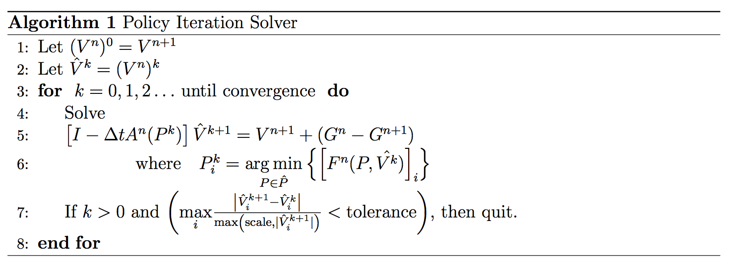
The $\arg\min$ term in line 6 of Algorithm (1) implements a linear search of the controls $P_h=\{p_1=0, p_2\ldots,p_J = p_{\text{max}}\}$, respecting the maximal use of central differencing as much as possible.
Python Finite Difference Implementation
We implement the method using the parameters in the table below,
| $r$ | $\sigma$ | $\xi$ | $\pi$ | $w_0$ | $T$ | $\gamma$ | $J$ | $p_{\text{max}}$ | $w_{\text{max}}$ |
|---|---|---|---|---|---|---|---|---|---|
| 0.03 | 0.15 | 0.33 | 0.1 | 1.0 | 20 | 14.47 | 8 | 1.5 | 5.0 |
import numpy as np
from   scipy.sparse import spdiags, identity
from   scipy.sparse.linalg import spsolve
import matplotlib.pyplot as plt
#from   bokeh.plotting import figure, output_notebook, show, gridplot, save
import pandas as pd

%matplotlib inline
#output_notebook()

CENTRAL =0
FORWARD =1
BACKWARD= 2

def main():
    r     = 0.03
    sigma = 0.15
    xi    = 0.33
    pi    = 0.1
    W0    = 1.0
    T     = 20.0
    gamma = 14.47
    Wmin  = 0.0
    Wmax  = 5.0
    M     = 1600
    N     = 100
    tol   = 1e-6
    scale = 1.0
    Pmax  = 1.5
    J     = 8

    hsigsq  = 0.5 * sigma ** 2 # half sigma squared -> 0.5 x sigma^2
    sigmaxi = sigma * xi
    dW      = ( Wmax - Wmin) / N
    dt      = T / M
    dWsq    = dW ** 2

    W    = np.linspace( Wmin, Wmax, N + 1 ) # need N+1 for there to be N steps between 0.0 and 5.0
    Ps   = np.linspace( 0.0, Pmax, J ) # discretize controls
    I    = identity( N + 1 )
    Gn   = np.zeros_like( W )
    Gnp1 = np.zeros_like( W )

    terminal_values = ( W - 0.5 * gamma ) ** 2

    def bc( t ): # boundary condition
        tau = T - t
        c   = ( 2 * pi ) / r

        e1 = np.exp( r * tau )
        e2 = np.exp( 2 * r * tau )
        alpha = e2 * ( Wmax**2 )
        beta  = ( c * e2 - ( gamma + c ) *e1 ) * Wmax
        delta = ( ( gamma**2 ) / 4.0 ) +  ( ( pi * c ) / ( 2 * r ) ) * ( e2 - 1 )\
                - ( ( pi * ( gamma + c ) ) / r ) * ( e1 - 1 )
        return alpha + beta + delta

    def alpha( W, p, dirn = CENTRAL ):
        t1 = hsigsq * (p**2) * (W**2) / dWsq
        t2 = ( pi + W * ( r + p * sigmaxi ) )
        if dirn == CENTRAL:
            return t1 - t2 / ( 2 * dW )
        elif dirn == BACKWARD:
            return t1 - t2 / dW
        elif dirn == FORWARD:
            return t1

    def beta( W, p, dirn = CENTRAL ):
        t1 = hsigsq * (p**2) * (W**2) / dWsq
        t2 = ( pi + W * ( r + p * sigmaxi ) )
        if dirn == CENTRAL:
            return t1 + t2 / (2 *dW)
        elif dirn == FORWARD:
            return t1 + t2 / dW
        elif dirn == BACKWARD:
            return t1

    def makeDiagMat( alphas, betas ):
        d0, dl, d2 = -( alphas + betas ), np.roll( alphas, -1 ), np.roll( betas, 1 )
        d0[-1] = 0.
        dl [-2:] = 0.
        data = np.array( [ d0, dl, d2 ] )
        diags = np.array( [ 0, -1, 1 ] )
        return spdiags( data, diags, N + 1, N + 1 )

    def find_optima1_ctrls( Vhat, t ):

        Fmin = np.tile( np.inf, Vhat.size )

        optdiffs = np.zeros_like( Vhat, dtype = np.int )
        optP    = np.zeros_like( Vhat )

        alphas  = np.zeros_like( Vhat ) # the final
        betas   = np.zeros_like( Vhat ) # the final
        curDiffs = np.zeros_like( Vhat, dtype = np.int )

        for p in Ps: # Hnd the optimal control
            alphas[:] = -np.inf
            betas[:] = -np.inf
            curDiffs[:] = CENTRAL

            for diff in [ CENTRAL, FORWARD, BACKWARD ]:
                a = alpha( W, p, diff)
                b = beta( W, p, diff )
                positive_coeff_indices = np.logical_and( a >= 0.0, b >= 0.0 ) == True
                positive_coeff_indices = np.logical_and( positive_coeff_indices, alphas==-np.inf )
                indices = np.where( positive_coeff_indices )

                alphas[ indices ] = a[ indices ]
                betas[ indices ] = b[ indices ]
                curDiffs[ indices ] = diff

            M = makeDiagMat( alphas, betas )
            F = M.dot( Vhat )
            indices = np.where( F < Fmin )

            Fmin[indices] = F[indices ]
            optP[indices] = p
            optdiffs[indices] = curDiffs[ indices ]
        return optP, optdiffs

    timesteps = np.linspace( 0.0, T, M + 1 )[:-1] # drop last item which is T=20.0
    timesteps = np.flipud( timesteps )
    V = terminal_values
    alphas = np.zeros_like( V )
    betas = np.zeros_like( V )

    for t in timesteps:

        Vhat = V.copy()
        Gnp1[-1] =bc(t+ dt)
        Gn[-1] = bc( t)
        B        = Gn - Gnp1 # new boundary cone - old boundary cone

        while True:
            ctrls, diffs = find_optima1_ctrls( Vhat, t )
            for diff in [ CENTRAL, FORWARD, BACKWARD ]:
                indices = np.where( diffs == diff )
                alphas[indices] = alpha( W[indices], ctrls[indices], diff )
                betas[indices] = beta( W[indices], ctrls[indices], diff )

            A   = makeDiagMat( alphas, betas )
            M = I - dt * A
            Vnew = spsolve( M, V + B )
            scale    = np.maximum( np.abs( Vnew ), np.ones_like( Vnew ) )
            residuals = np.abs( Vnew - Vhat ) / scale
            if np.all( residuals[:-1] < tol ):
                V = Vnew
                break
            else:
                Vhat = Vnew

    return W, V, ctrls

W, V, ctrls = main()
f, (ax1, ax2) = plt.subplots(1, 2, figsize=(16,5))
ax1.plot(W, V, color = 'pink', lw=2)
ax1.set_title('Plot of $V(W=w_0, 0)$ against wealth')
ax2.plot(W, ctrls, color = 'orange', lw=2, alpha = 0.7)
_ = ax2.set_title('Plot of optimal control against wealth')

In the above, we show plots of $V(W=w_0, 0)$ and the optimal control against wealth that was derived from the finite difference solution.
Conclusion
We have given a concise review of the theory of continuous-time mean-variance portfolio selection, and shown how the policy-iteration algorithm can be efficiently implemented in Python with the use of Numpy/Scipy.
References
[1] Zhou, X. and D. Li (2000). Continuous time mean variance portfolio selection: A stochastic LQ framework. Applied Mathematics and Optimization 42, 19–33.
[2] Wang, J. and P. A. Forsyth (2010). Numerical solution of the Hamilton Jacobi Bellman formulation for continuous time mean variance asset allocation. Journal of Economic Dynamics and Control 34 (2), 207–230.
[3] Wang, J. and P. Forsyth (2008). Maximal use of central differencing for Hamilton-Jacobi-Bellman PDEs in finance. SIAM Journal on Numerical Analysis 46, 1580–1601.
Appendix
Solution to the PDE in $(3)$.
The derivatives of $\alpha(\tau)$, $\beta(\tau)$, $\delta(\tau)$ are,
$$ \begin{aligned} \alpha^\prime(\tau) &= 2r \exp( 2r\tau)\\ \beta^\prime(\tau) &= -r(\gamma + c )\exp(r\tau) + 2rc\exp(2r\tau)\\ \delta^\prime(\tau) &= -\pi(\gamma+c)\exp(r\tau) + \pi c\exp( 2r\tau) \end{aligned} $$Assume that the solution is given by,
$$ V(w, T-\tau) = \alpha(\tau) w^2 + \beta(\tau)w + \delta(\tau) $$Then we have,
$$ \begin{aligned} \frac{\partial V}{\partial t} &= \frac{\partial V}{\partial \tau } \frac{\partial \tau}{\partial t}\\ &= -\frac{\partial V}{\partial \tau }\\ &=-\alpha^\prime(\tau)w^2 - \beta^\prime(\tau) w - \delta^\prime(\tau)\\ &= -2rw^2 \exp( 2r\tau) + rw(\gamma+c)\exp(r\tau)-2rcw\exp(2r\tau)\\ & \quad\,+\pi(\gamma+c)\exp(r\tau) - \pi c\exp( 2r\tau)\\ &= (\pi+rw)(\gamma+c)\exp(r\tau)-( 2rw^2 + 2rcw + \pi c )\exp(2r\tau) \end{aligned} $$For the term involving the partial derivative of $V$ with respect to $W$,
$$ \begin{aligned} (\pi+rw)\frac{\partial V }{\partial w}&= (\pi + rw ) ( 2w\alpha(\tau) + \beta(\tau))\\ &=(\pi + rw ) ( 2w \exp(2r\tau)-(\gamma+c)\exp(r\tau)+c\exp(2r\tau))\\ &= -(\pi + rw )(\gamma+c)\exp(r\tau) + (\pi + rw )(2w + c)\exp(2r\tau) \end{aligned} $$With the above together we have,
$$ \begin{aligned} \frac{\partial V}{\partial t} + (\pi+rw)\frac{\partial V }{\partial w}&=(\pi+rw)(\gamma+c)\exp(r\tau)-( 2rw^2 + 2rcw + \pi c )\exp(2r\tau)\\ &\quad\,-(\pi + rw )(\gamma+c)\exp(r\tau) + (\pi + rw )(2w + c)\exp(2r\tau)\\ &=[-(2rw^2 + 2rcw + \pi c) + (2rw^2+rcw + \pi c + 2\pi w)]\exp(2r\tau)\\ &= (-rcw + 2\pi w ) \exp(2r\tau)\\ &= (-2\pi w + 2\pi w ) \exp(2r\tau)\\ &=0 \end{aligned} $$Therefore, we have shown that $V(w, T-\tau) = \alpha(\tau) w^2 + \beta(\tau)w + \delta(\tau)$ is a solution to the PDE in $(3)$, which is the boundary condition for large $w$.